Convolutional Layers
In a multi-layer perceptron, every neuron composes a linear combination of its inputs with a nonlinear function. We call a layer of such neurons fully-connected, because every neuron is connected to every input, or to the output of every neuron in the preceding layer. Fully connected layers have the advantage that their neurons can respond to patterns that might span the entire input. We say that they respond to global features. Fully-connected layers have the disadvantage of requiring a numerous parameters or weights (a number equal to the product of the number of inputs and the number of outputs).
For computer vision problems (like classification of the MNIST dataset) scientists intuited the importance of local features, features that spanned only a small region of an image. This intuition was supported by Hubel and Weisel’s study of the cat’s visual cortex, in which they observed that individual neurons responded to a band of light in a specific location and orientation.
In a two-dimensional convolutional layer, each neuron is only connected to a subset of its inputs. The subset is not random or scattered—it is a small, square region of the input image. The process is illustrated in the online book, Neural Networks and Deep Learning:
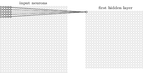
Each neuron in the layer is connected to a different region of the input. However, the regions may overlap. Furthermore, each neuron is constrained to have the same weights as every other. In other words, the neurons in a convolutional layer are identical except for the region of the input they are connected to. As a result, the neurons learn to detect one local feature, and the layer becomes a feature map, describing where in the image that feature occured.
The multi-layer perceptron had a layer that looked for 500 different features, each across the entire input. Similarly, in practice, numerous two-dimensional convolutional layers are used for the same input, each mapping a different feature.
It should be noted that this topology introduces many calculations during forward propagation, to generate feature maps. However, because a single neuron’s parameters are used throughout a feature map, a comparitively small number of weights is introduced. Consequently, the number of gradients to be calculated during backpropagation is also quite small.